Flow Matching: A Minimal Guide

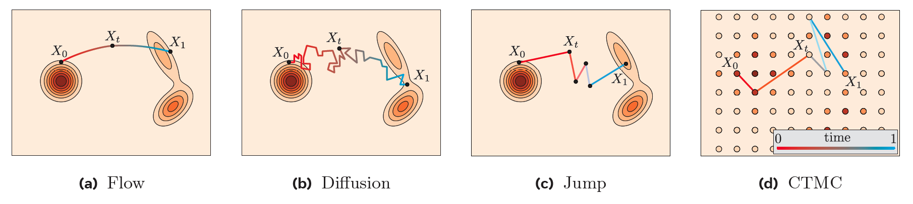
Flow Matching (FM) (Lipman et al., 2023) has seen impressive success in image and video generation [Link]. The key idea is to train a neural network to learn the underlying vector (velocity) field that deterministically pushes particles along this transport path.

Continuous State Space

Problem setup

Consider a vector field \(\mathrm{v_t : \mathbb{R}^d \to \mathbb{R}^d}\) and define its flow map \(\mathrm{\phi_t}\) as the solution of the ODE

Let \(\mathrm{p_0}\) and \(\mathrm{p_1}\) be the prior and data distributions, respectively. The marginal probability \(\mathrm{p_t:=[\phi_t]_\# p_0}\) is defined as the pushforward of \(\mathrm{p_0}\) under \(\mathrm{\phi_t}\). Equivalently, by change-of-variables [Link]:

The marginal probability \(\mathrm{p_t}\) satisfies the continuity equation (see Theorem 1 (Chen et al., 2018)):

To approximate the true vector field \(\mathrm{v_t(x)}\) via a parameterize \(\mathrm{v_{\theta}(t, x)}\), the ideal regression loss is:

This is, however, intractable, since both \(\mathrm{p_t}\) and \(\mathrm{v_t}\) are unknown.

Conditional Flow Matching (CFM)

To make the loss more tractable, we introduce a conditioning variable \(\mathrm{x_1\sim p_1}\) and define a conditional flow map \(\mathrm{\psi_t(\cdot \mid x_1)}\) along with a conditional vector field \(\mathrm{v_t(x \mid x_1)}\) satisfying

The unconditional velocity field can then be expressed as a conditional expectation:

Recall that \(\mathrm{\psi_t}\) pushes the prior distribution from $\mathrm{p_0}$ to $\mathrm{p_t(\cdot\mid x_1)}$ in \eqref{map_psi}. We can re-define the CFM loss:

By regressing \(\mathrm{v_{\theta}}\) to match the conditional vector field, we obtain an unbiased estimator of the FM loss.

Special Flow Maps

Consider a map \(\mathrm{\psi_t(x\mid x_1)} \mathrm{=\sigma_t(x_1) x + \mu_t(x_1)}\). Taking time gradient and combining Eq.\eqref{flow_eqn}, we have

Replacing $\mathrm{\psi_t(x \mid x_1)}$ with $\mathrm{x}$, s.t. \(\mathrm{\psi_t(x \mid x_1):=\dfrac{x-\mu_t(x_1)}{\sigma_t(x_1)}}\), we have

Connections to Diffusion Models: For VE-SDE (Song et al., 2021), we have \(\mathrm{p_t(x)=N(x\mid x_1, \sigma_{1-t}^2I)},\) the conditional vector field follows \(\mathrm{v_t(x\mid x_1)=-\frac{\sigma_{1-t}'}{\sigma_{1-t}}(x-x_1)}\) via Eq.\eqref{vector_field_formula}. For VP-SDE, the conditional probability follows \(\begin{equation} \mathrm{p_t(x \mid x_1) = N\!\left( x \,\middle|\, \alpha_{1-t} x_1,\, (1 - \alpha_{1-t}^2) I \right)}\notag \end{equation}\), where \(\mathrm{\alpha_t = e^{-\tfrac{1}{2}\int_0^t \beta(s)\,ds}}\). The vector field can be derived in the same way.

Connections to Optimal Transport (OT): Consider the OT flow map:

which corresponds to a displacement map \(\mathrm{p_t=[(1-t)id+t\psi]_* p_0}\). The conditional vector field follows \(\mathrm{v_t(x\mid x_1)=\dfrac{x_1-x}{1-t}}\). The simplified CFM loss function follows that

Network Parameterization

In diffusion models, noise prediction (Song et al., 2021) learns to predict the added noise \(\mathrm{v_t(x \mid x_0)=p_t(x\mid x_0)}\), while data prediction (Karras et al., 2022) learns to recover the clean data \(\mathrm{v_t(x \mid x_1)=p_t(x\mid x_1)}\) directly. They’re mathematically equivalent, but the denoiser view often makes training more stable and easier to control.

Discrete State Spaces

Problem setup

Consider a sequence \(\mathrm{x=\{x^1, \cdots, x^d\}\in \mathcal{S}}\), where $\mathcal{S}$ is the discrete state space, $\mathrm{x^i\in \mathcal{V}}$ is a token or coordinate and \(\mathcal{V}\) is a vocabulary \(\mathrm{\{1, 2, \cdots, V\}}\). We define the sequence-level \(\mathrm{\delta(x,y)=1}\) if \(\mathrm{x=y}\) and 0 otherwise. It is also used in token-level s.t. \(\mathrm{\delta(x^i, y^i)}\) for some \(\mathrm{x^i, y^i\in \mathcal{V}}\).

Continuous-time Markov Chain (CTMC)

For a CTMC, a random variable \(\mathrm{(X_t)_{0\leq t\leq 1}}\) induces a transition kernel \(\mathrm{p_{t+h\mid t}}\) defined as

where $\mathrm{v_t(y, x)}$ denotes the transition rate or velocity field from state \(\mathrm{x\in \mathcal{S}}\) to \(\mathrm{y\in \mathcal{S}}\):

The marginal probability \(\mathrm{p_t}\) for the random variable \(\mathrm{(X_t)_{0\leq t\leq 1}}\) satisfy the Kolmogorov forward equation

State Transitions with At-most One Token

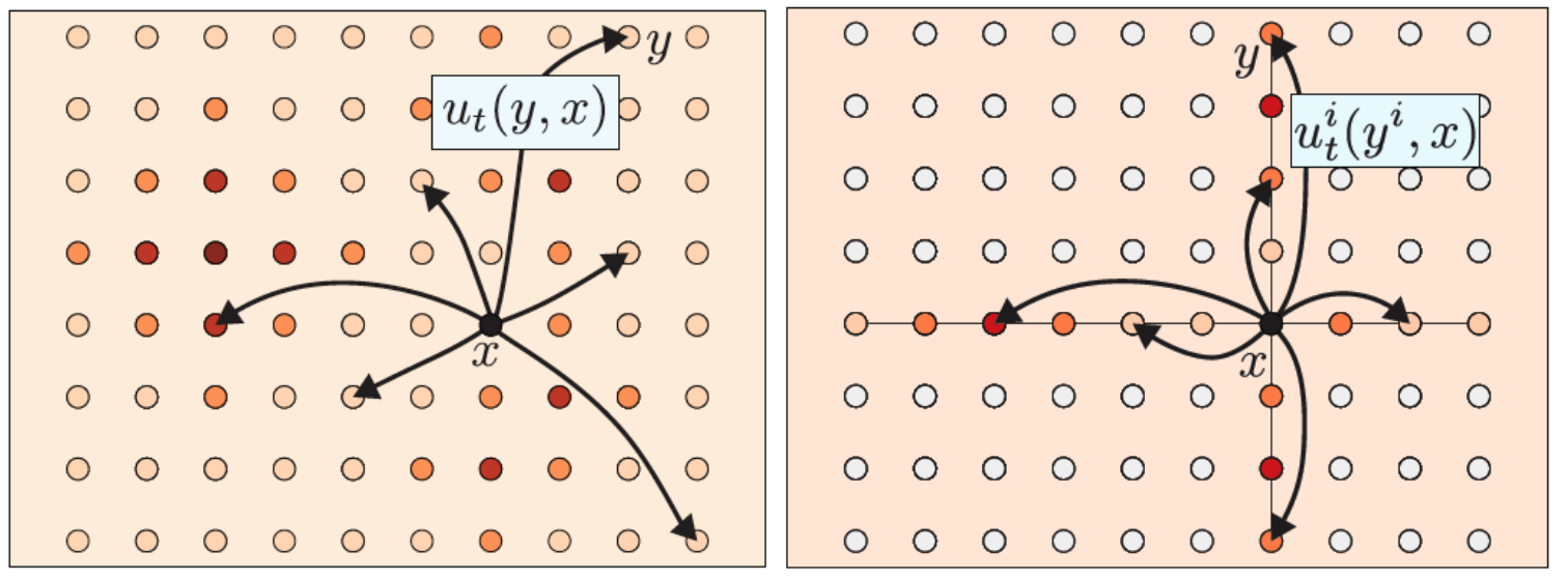
Note that naïve transitions from \(\mathrm{x}\) to all possible states \(\mathrm{y}\) results in a huge output dimension \({\mathrm{\textbf{V}^d}}\). we introduce factorized velocities that only allow transitions affecting at most one token:

where \(\mathrm{\bar i=(1, \cdots, i-1, i+1, \cdots, d)}\). It thus suffices to model \(\mathrm{v_t^i(y^i, x)}\) instead of \(\mathrm{v_t(y, x)}\) and the modeling complexity is significantly reduced from \({\mathrm{\textbf{V}^d}}\) to \({\mathrm{\textbf{V}d}}\).

Given \(\mathrm{X_0\sim p_0}\) and the factorized paths and velocities, we can sample \(\mathrm{X_t}\) using the Euler method

where the last equality follows from \(\mathrm{\prod_i (a^i + hb^i)=\prod_i a^i + h\sum_i \big(\prod_{j\neq i} a^j\big)b^i + o(h)}\).

Conditional Velocity

Analogous to the continuous case, (Gat et al., 2024) introduced the conditional velocity field s.t.

where \(\mathrm{p_{0, 1\mid t}(x_0, x_1\mid x)=\dfrac{p_{t\mid 0, 1}(x\mid x_0, x_1) p_{X_0, X_1}(x_0, x_1)}{p_t(x)}}\).

The factorized conditional path assumes that

where each \(\mathrm{p_{t\mid 0, 1}^i (x^i \mid x_0, x_1)}\) follows an interpolation schedule \(\mathrm{(\kappa_t)_{t\in[0, 1]}}\) and \(\mathrm{\kappa_0=0, \kappa_1=1}\)

A random variable \(\mathrm{X_t^i\sim p_{t\mid 0, 1}^i}\) follows

The dynamics of the conditional marginal probability \(\mathrm{p_t^i}\) then satisfies (Lipman et al., 2024)

Thus, the conditional velocity follows by Eq.\eqref{v_def}

However, constructing probability-preserving velocities remains challenging and typically requires additional learning of \(\mathrm{p_{0\mid t}^i}\) (Lipman et al., 2024).

Velocity Parameterization

where \(\mathrm{p^i_{1\mid t}(x_1 \mid x)=\sum_{x_0, x_1^{\bar i}} p_{0, 1\mid t}(x_0, x_1 \mid x)=\mathbb{E}\big[\delta(x_1^i, X_1^i)\mid X_t=x\big]}\).

Hence, one may learn \(\mathrm{v_t^i(y^i, x)}\) via a parametrized model \(\mathrm{p_{1\mid t}^{\theta, i}(x_1^i\mid x)}\) as the data prediction. A suitable conditional matching loss is

Citation

@misc{deng2025flowmatching,
  title   ={{Flow Matching: A Minimal Guide}},
  author  ={Wei Deng},
  journal ={waynedw.github.io},
  year    ={2025},
  howpublished = {\url{https://www.weideng.org/posts/flow_matching/}}
}