Generalized Reparametrization Tricks
Backpropagation of continuous and discrete random variables
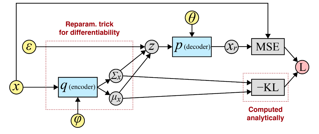
Suppose we are interested in the marginal likelihood $\mathrm{p_{\theta}(x)}$. Consider a latent representation via variational autoencoder (VAE) (Kingma & Welling, 2013)
\[\begin{align} \mathrm{\log p_\theta(\mathbf{x})} &= \mathrm{\log \int p_\theta(\mathbf{x}, \mathbf{z}) \, d\mathbf{z}} \notag \\ &= \mathrm{\log \int q_\phi(\mathbf{z} \mid \mathbf{x}) \frac{p_\theta(\mathbf{x}, \mathbf{z})}{q_\phi(\mathbf{z} \mid \mathbf{x})} \, d\mathbf{z}} \notag \\ &\geq \mathrm{\mathbb{E}_{q_\phi(\mathbf{z} \mid \mathbf{x})} \log \frac{\overbrace{p_\theta(\mathbf{x}, \mathbf{z})}^{p_\theta(\mathbf{z}) p_\theta(\mathbf{x}\mid \mathbf{z})}}{q_\phi(\mathbf{z} \mid \mathbf{x})}} \notag \\ &=\mathrm{-D_{\mathrm{KL}}\left( q_\phi(\mathbf{z} \mid \mathbf{x}) \,\|\, p(\mathbf{z})\right)+\mathbb{E}_{q_\phi(\mathbf{z} \mid \mathbf{x})} \left[ \log p_\theta(\mathbf{x} \mid \mathbf{z}) \right]}, \notag \end{align}\]where $\geq$ follows from Jensen’s inequality, \(\mathrm{q_\phi(\mathbf{z} \mid \mathbf{x})}\) is the encoder, and \(\mathrm{p_\theta(\mathbf{x} \mid \mathbf{z})}\) is the decoder.
We denote the integrand by $\mathrm{f_\phi(\mathbf{z})}$ and write $\mathrm{q_\phi(\mathbf{z} \mid \mathbf{x})}$ simply as $\mathrm{q_\phi(\mathbf{z})}$. To optimize the loss function via backpropagation, the gradient of \(\mathrm{\mathbb{E}_{q_\phi(\mathbf{z})}[f_\phi(\mathbf{z})]}\) w.r.t. $\phi$ follows
\[\begin{align} \mathrm{\nabla_\phi \mathbb{E}_{q_\phi(\mathbf{z})}[f_\phi(\mathbf{z})] } &= \mathrm{\int_{\mathbf{z}} \nabla_\phi \left[ q_\phi(\mathbf{z}) f_\phi(\mathbf{z}) \right] \, d\mathbf{z} = \underbrace{\int_{\mathbf{z}} f_\phi(\mathbf{z}) \nabla_\phi q_\phi(\mathbf{z}) \, d\mathbf{z}}_{\text{Intractable if $q_\phi(\mathbf{z})\neq 0$}} + \mathbb{E}_{q_\phi(\mathbf{z})} \left[ \nabla_\phi f_\phi(\mathbf{z}) \right]}. \notag \end{align}\]We observe that the first term in RHS suffers from the large variance issue and is not differentiable.
Continuous Variables
Introducing a deterministic mapping $\mathrm{g_\phi:\mathbf{z} = g_\phi(\boldsymbol{\epsilon})}$, where $\boldsymbol{\epsilon} \sim q(\boldsymbol{\epsilon})$ (e.g. Gaussian) gives
\[\begin{align} \mathrm{\nabla_\phi \mathbb{E}_{q_\phi(\mathbf{z})}[f(\mathbf{z})] } &= \mathrm{\nabla_\phi \mathbb{E}_{q(\boldsymbol{\epsilon})}\left[ f\left(g_\phi(\boldsymbol{\epsilon})\right) \right] \approx \frac{1}{L} \sum_{l=1}^L \nabla_\phi f\left(g_\phi(\boldsymbol{\epsilon}^{(l)})\right)}, \notag \end{align}\]which is the well-known reparametrization trick in VAEs. For simplicity, the Gaussian distribution can be a multivariate Gaussian with a diagonal covariance structure.
We further note that this one-step mapping from the data distribution to a Gaussian offers insight into the iterative transformations in diffusion models (Song et al., 2021).
Discrete Variables
When the latent variable $z$ in VAEs is a k-class categorical distribuion, the Gumbel-Max trick (Gumbel, 1954) proposes to draw samples $\mathbf{z}$ from a categorical distribution with k-class probabilities $\boldsymbol{\pi}$:
\[\begin{equation} \mathrm{\mathbf{z} = \mathrm{\text{one_hot}} \left( \arg\max_i \left[ g_i + \log \pi_i \right] \right)} \notag, \end{equation}\]where $\mathrm{g_1, \dots, g_k}$ are i.i.d. samples drawn from $\mathrm{Gumbel}(0, 1)$ link.
The Gumbel distribution is commonly used to model the distribution of the maximum (or minimum) of samples, with its CDF $\mathrm{F(x)=e^{-e^{-x}}}$. Invoking the inverse CDF trick, it is equivalent to drawing $\mathrm{-\log(-log(u_i))}$, where $\mathrm{u_i\sim Uniform(0, 1)}$.
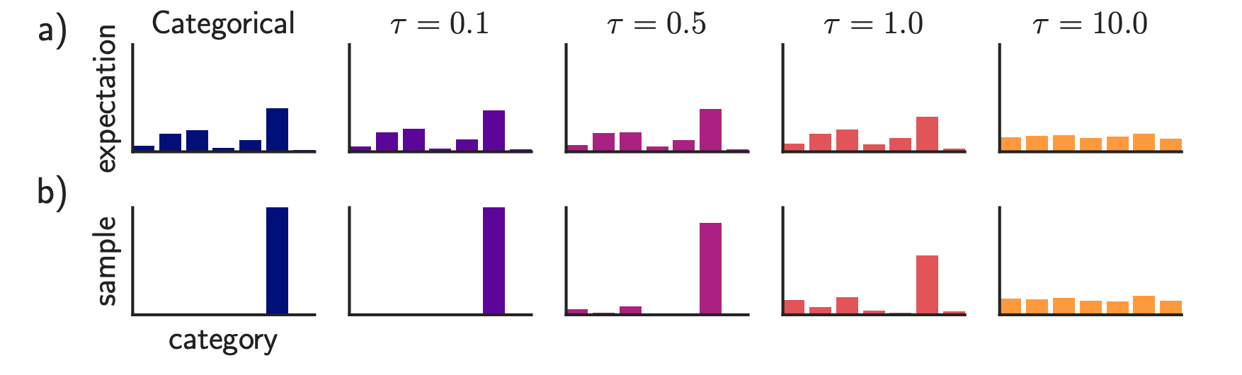
To enable a differentiable approximation, (Jang et al., 2017) proposed a softmax relaxation s.t.
\[\begin{equation} \mathrm{\mathbf{z}_i \approx \frac{\exp\left((\log \pi_i + g_i)/\tau\right)}{\sum_{j=1}^k \exp\left((\log \pi_j + g_j)/\tau\right)}, \quad \text{for } i = 1, \dots, k .}\notag \end{equation}\]Despite its simplicity and the absence of high-variance gradients, Gumbel–Softmax introduces a nontrivial bias. To further mitigate this issue, one can instead follow REINFORCE (Williams, 1992) and differentiate through the underlying probability distribution directly. We discuss this perspective in more detail in this [Blog].
Citation
@misc{deng2025_preparmetrization_tricks,
  title   ={{Generalized Reparametrization Tricks}},
  author  ={Wei Deng},
  journal ={waynedw.github.io},
  year    ={2025},
  howpublished = {\url{https://www.weideng.org/posts/reparamet_tricks/}}
}
- Kingma, D. P., & Welling, M. (2013). Auto-Encoding Variational Bayes. ArXiv Preprint ArXiv:1312.6114.
- Song, Y., Sohl-Dickstein, J., P. Kingma, D., Kumar, A., Ermon, S., & Poole, B. (2021). Score-Based Generative Modeling through Stochastic Differential Equations. International Conference on Learning Representations (ICLR).
- Gumbel, E. J. (1954). Statistical theory of extreme values and some practical applications: a series of lectures (Number 33). US Govt. Print. Office.
- Jang, E., Gu, S., & Poole, B. (2017). Categorical Reparameterization with Gumbel-Softmax. Proceedings of the 5th International Conference on Learning Representations (ICLR).
- Williams, R. J. (1992). Simple statistical gradient-following algorithms for connectionist reinforcement learning. Machine Learning, 8(3–4), 229–256.