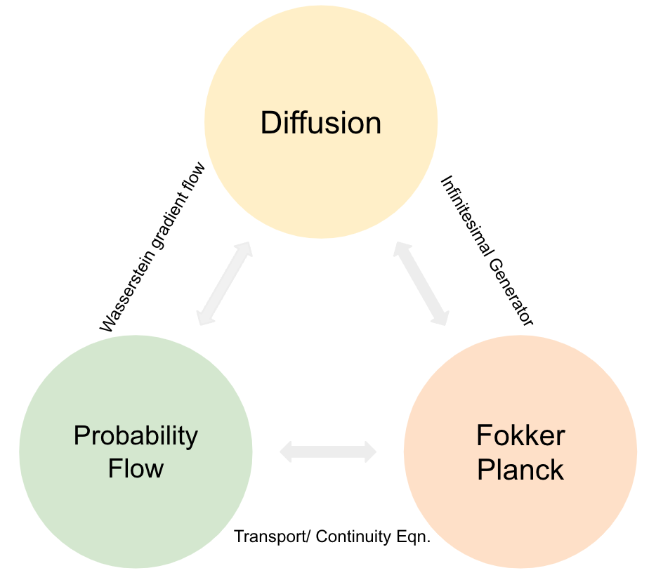
The Triangle of Flow, Diffusion, and PDE
Connections between Probability Flows, Diffusions, and PDEs.
Diffusion Process
Consider a diffusion process that solves the Itô’s SDE (Øksendal, 2003):
\[\begin{align} \mathrm{d} \mathrm{X}_t=\boldsymbol{\mathrm{v}_t}(\mathrm{X}_t) \mathrm{d} t + \sigma(X_t) \mathrm{d} \mathrm{W}_t.\label{SDE} \end{align}\]Denote by $\mathrm{P}_t$ the transition function of Markov process
\[\begin{align} (\mathrm{P}_t f)(x)=\int f(y)\mathrm{P}(t, x, \mathrm{d} y)\notag. \end{align}\]We can easily check that $\mathrm{P}_t$ is a linear operator and an example of a Markov semigroup.
Define the generator $\mathscr{L}f=\lim \frac{\mathrm{P}_t f - f}{y}$, where $\mathrm{P}_t=e^{t \mathscr{L}}$. Analyzing the transition of the conditional expectation $\mathbb{E}(f(\mathrm{X}_t)|\mathrm{X}_s=x)$ for a bounded function $f$ (Ito’s formula), where $s\leq t$, we have the backward Kolmogorov equation
\[\begin{align} \mathscr{L}&=\boldsymbol{\mathrm{v}}\cdot \nabla + \frac{1}{2} \Sigma:D^2\notag\\ &=\sum_{j=1}^d \mathrm{v}_j\frac{\partial}{\partial x_j} + \frac{1}{2}\sum_{i,j=1}^d \Sigma_{ij}\frac{\partial^2}{\partial x_i \partial x_j}\notag. \end{align}\]where $\nabla$ and $\nabla\cdot$ denote the gradient and the divergence in $\mathbb{R}^d$, $\Sigma(x)=\sigma(x) \sigma(x)^\intercal$ and $D^2$ denotes the Hessian matrix.
Fokker-Planck PDE
Further define the semigroup $\mathrm{P}_t^{*}$ that acts on probability measures
\[\begin{align} \mathrm{P}^{*}_t \mu(\Gamma)=\int \mathrm{P}(t, x, \Gamma)\mathrm{d} \mu(x)\notag. \end{align}\]The semigroup $\mathrm{P}_t$ and $\mathrm{P}_t^{*}$ are adjoint in $L^2$ such that
\[\begin{align} \int (\mathrm{P}_t f)\mathrm{d}\mu=\int f\mathrm{d}(\mathrm{P}_t^{*}\mu)\notag, \end{align}\]which yields
\[\begin{align} \int \mathscr{L} f h \mathrm{d} x = \int f \mathscr{L}^* h \mathrm{d}x, \text{ where } \mathrm{P}_t^*=e^{t {\mathscr{L}}^*}.\notag \end{align}\]Let $p_t$ denote the law of the Markov process at time $t$. The law of $p_t$ follows that
\[\begin{align} \frac{\partial p_t}{\partial t} =\mathscr{L}^* p_t,\notag \end{align}\]which is the Fokker-Planck equation (FKP), also known as forward Kolmogorov equation. Analyzing the evolution of the probability densities, we have
\[\begin{align} \mathscr{L}^{*} p_t&=\nabla \cdot \bigg(-\boldsymbol{\mathrm{v}} p_t + \frac{1}{2} \nabla\cdot\big(\Sigma p_t\big)\bigg). \notag \\ &=\nabla \cdot \bigg(-\boldsymbol{\mathrm{v}} p_t + \frac{1}{2} \big(\nabla\cdot \Sigma\big) p_t + \frac{1}{2} \Sigma \nabla p_t \bigg). \notag \\ &=\nabla \cdot \bigg(-\underbrace{\bigg(\boldsymbol{\mathrm{v}} - \frac{1}{2} \big(\nabla\cdot \Sigma\big) - \frac{1}{2} \Sigma \nabla \log p_t\bigg)}_{\boldsymbol{\nu}_t} p_t \bigg), \label{FPE} \\ \end{align}\]where the last equality follows by $\nabla \log p_t = \frac{\nabla p_t}{p_t}$. One can easily derive a backward Kolmogorov equation from a forward Kolmogorov equation by invoking the integration by parts, e.g. Eq.(15) of (Chen et al., 2023).
Probability Flow
Denote by $\boldsymbol{\nu}=\boldsymbol{\mathrm{v}} - \frac{1}{2} \big(\nabla\cdot \Sigma\big) - \frac{1}{2} \Sigma \nabla \log p$, the FPE is recased as the transport equation (Santambrogio, 2015) or continuity equation in fluid dynamics (Chewi, 2023).
\[\begin{align} \partial_t p_t =- \nabla \cdot ({\boldsymbol{\nu_t}} p_t).\label{ODE} \end{align}\]Interestingly, it corresponds to the probability flow ODE (Song et al., 2021)
\[\begin{align} \mathrm{d} X_t={\boldsymbol{\nu_t}}(X_t) \mathrm{d} t.\notag \end{align}\]Apply the instantaneous change of variables (Chen et al., 2018), the log-likelihood of $p_0(x)$ follows that
\[\begin{align} \log p_0(x)=\log p_T(x) + \int_0^T \nabla \cdot {\boldsymbol{\nu_t}} \mathrm{d} t,\notag \end{align}\]which provides an elegant way to compute the likelihood for diffusion models.
In practice, it is expensive to evaluate the divergence $\nabla \cdot {\boldsymbol{\nu_t}}$. We can adopt the Hutchinson trace estimator (Hutchinson, 1989).
\[\begin{align} \nabla \cdot {\boldsymbol{\nu_t}} = \mathbb{E} \big[\epsilon^\intercal \nabla {\boldsymbol{\nu_t}} \epsilon \big],\notag \end{align}\]where $\nabla \cdot {\boldsymbol{\nu_t}}$ is the Jacobian of ${\boldsymbol{\nu_t}}$; the random variable $\epsilon$ is a standard Gaussian vector and $\epsilon^\intercal \nabla {\boldsymbol{\nu_t}}$ can be efficiently computed using reverse-mode automatic differentiation.
Wasserstein Gradient Flow
Consider a homogeneous case where $\boldsymbol{\mathrm{v_t}}\equiv -\nabla \mathrm{V}$ and $\Sigma(x)=2\boldsymbol{\text{I}}$ for Eq.\eqref{SDE}, the vector field $\boldsymbol{\nu}$ can be interpreted as the tangent vector for the curves of measures $t\rightarrow p_t$ (Richard Jordan, 1998) (Chewi, 2023). Define a functional $\mathcal{F}=\text{KL}(\cdot||\pi)$, where $\pi\propto \exp(-\mathrm{V})$. We have
\[\begin{align} \mathcal{F}(p)=\int p \log \frac{p}{\pi} = \int p \mathrm{V} + \int p \log p.\notag \end{align}\]Taking the first variation of $\mathcal{F}$ at $p$, we have
\[\begin{align} \delta \mathcal{F}(p)= \mathrm{V} + \log p+\text{constant}.\notag \end{align}\]The Wasserstein gradient at $p$ follows that
\[\begin{align} \nabla_{\text{W}_2} \mathcal{F}(p):=\nabla \delta \mathcal{F}(p)= \nabla \mathrm{V} + \nabla\log p=-\boldsymbol{\nu},\notag \end{align}\]where the last equality follows by Eq.\eqref{FPE}.
Now the transport equation \eqref{ODE} can be also formulated as the Wasserstein gradient flow of $\mathcal{F}$
\[\begin{align} \partial_t p_t =\nabla \cdot \bigg(\nabla_{\text{W}_2} \mathcal{F}(p_t) p_t\bigg).\notag \end{align}\]The following is a demo that describes the connections:

Acknowledge
Big thanks to my friend Jiang Nan for helping build this website!
- Øksendal, B. (2003). Stochastic Differential Equations: An Introduction with Applications. Springer.
- Chen, Y., Deng, W., Fang, S., Li, F., Yang, N., Zhang, Y., Rasul, K., Zhe, S., Schneider, A., & Nevmyvaka, Y. (2023). Provably Convergent Schrödinger Bridge with Applications to Probabilistic Time Series Imputation. ICML.
- Santambrogio, F. (2015). Optimal Transport for Applied Mathematicians: Calculus of Variations, PDEs, and Modeling. Springer.
- Chewi, S. (2023). Log-Concave Sampling. Online Draft.
- Song, Y., Sohl-Dickstein, J., Kingma, D. P., Kumar, A., Ermon, S., & Poole, B. (2021). Score-Based Generative Modeling through Stochastic Differential Equations . ICLR.
- Chen, R. T. Q., Rubanova, Y., Bettencourt, J., & Duvenaud, D. (2018). Neural Ordinary Differential Equations. Neurips.
- Hutchinson, M. F. (1989). A Stochastic Estimator of the Trace of the Influence Matrix for Laplacian Smoothing Splines. Communications in Statistics-Simulation and Computation, 18(3), 1059–1076.
- Richard Jordan, F. O., David Kinderlehrer. (1998). The Variational Formulation of the Fokker-Planck Equation. SIAM Journal on Mathematical Analysis.